Thursday, November 15, 2007

Wednesday, November 14, 2007
Phase Transitions and Chemical Potentials
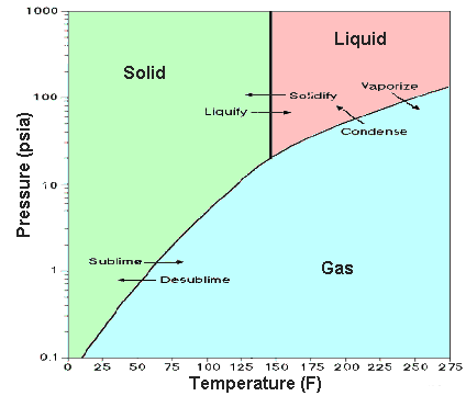
A substance's phase diagram tells us at what temperatures and pressures we will observe the six common phase transitions [fusion, freezing, vaporization, condensation, sublimation, deposition]. The triple point, where all three common phases are in mutual equilibrium, is a convenient phase transition marker: below it, you will typically see sublimation/deposition as temperature is changed and above it, vaporization/sublimation. When more than one crystalline form exists in the solid phase, more than one triple point is possible.
To truly understand phase transitions, we can plot the chemical potential μ vs T. Since (∂μ/∂T)P=–Sm, it is apparent that these plots trend downwards, and the slope cusps at the transition temperature. Where the solid and liquid lines intersect will be the substance's melting point (μS=μL). In fact, we can take this statement as the thermodynamic definition of the melting point. Analogously, the boiling point is that temperature at which the chemical potential of the liquid phase equals that of the vapor phase.
Pressure effects on the transition temperatures can be seen from the relationship (∂μ/∂P)T=Vm. Clearly an increase in pressure will similarly increase the chemical potential and the magnitude of this change is proportional to that phases molar volume. This leads to a boiling point elevation and freezing point elevation for most substances; in water, however, whose molar volume of solid is greater than that of the liquid phase, we see a freezing point depression as pressure is increased (as at the bottom of the ocean).
Since chemical potentials are equal for two phases in equilibrium, we are able to quickly derive the Clapeyron equation [dP/dT = ∆transS/∆transV] and its sister, the Clausius-Clapeyron equation: [dP/dT = ∆transH/T∆transV]. The latter equation allows us to easily obtain, in mathematical form, general formulas for the SL, LG and SG coexistence curves.
Chemical potential is a BIG idea in chemical thermodynamics – more for you to love! – and esplaining phase transitions is another eye-watering demonstration of the mad POWER of thermo.
To truly understand phase transitions, we can plot the chemical potential μ vs T. Since (∂μ/∂T)P=–Sm, it is apparent that these plots trend downwards, and the slope cusps at the transition temperature. Where the solid and liquid lines intersect will be the substance's melting point (μS=μL). In fact, we can take this statement as the thermodynamic definition of the melting point. Analogously, the boiling point is that temperature at which the chemical potential of the liquid phase equals that of the vapor phase.
Pressure effects on the transition temperatures can be seen from the relationship (∂μ/∂P)T=Vm. Clearly an increase in pressure will similarly increase the chemical potential and the magnitude of this change is proportional to that phases molar volume. This leads to a boiling point elevation and freezing point elevation for most substances; in water, however, whose molar volume of solid is greater than that of the liquid phase, we see a freezing point depression as pressure is increased (as at the bottom of the ocean).
Since chemical potentials are equal for two phases in equilibrium, we are able to quickly derive the Clapeyron equation [dP/dT = ∆transS/∆transV] and its sister, the Clausius-Clapeyron equation: [dP/dT = ∆transH/T∆transV]. The latter equation allows us to easily obtain, in mathematical form, general formulas for the SL, LG and SG coexistence curves.
Chemical potential is a BIG idea in chemical thermodynamics – more for you to love! – and esplaining phase transitions is another eye-watering demonstration of the mad POWER of thermo.
Monday, November 12, 2007
K's and Phase Transitions
On Friday's lecture, we discussed how the equilibrium constant K for a given reaction might change as we vary either the temperature or the pressure. From the Gibbs-Helmholtz equation, (∂(∆G/T)/∂T)P = – ∆H/T2 and that ∆G° = – RT lnK, it is straightforward to show that (∂(lnK)/∂T)P = ∆H°/RT2.
To see the effect of pressure, we look at the derivative (∂(∆G°)/∂P)T =∆V°. But, since the reference point ∆G° (1 bar) is independent of pressure, this derivative is zero and the dependence of K on P to be zero.
From these two results we conclude:
a) K is dependent only on temperature changes
b) this response is very sensitive (it is ln K that changes with T) and
c) the sign of the response is dictated by ∆H° (LeChatelier's principle in disguise)
Lastly, we began a formal discussion on phase diagrams/changes, our last chapter of the quarter, with the Ehrenfest classification of phase transitions. Some phase changes exhibit a discontinuity in the Sm vs T plot (as well as the Vm vs T plot). Since Sm is the first derivative of Gm, we call these first-order transitions. In other phase changes, the discontinuity does not arise until a plot of CP,m vs T; this is the second derivative of Gm so we call these second-order transitions. In general, an nth-order phase transition would have a discontinuity in the nth derivative of Gm, but only first and second-order are seen in practice. Though now outdated, the Ehrenfest classification is a useful way to think about the differences in the thermodynamics variables seen as systems undergo phase changes.
On Wednesday, phase diagrams and coexistence curves before hitting the Clausius-Clapeyron equation.
To see the effect of pressure, we look at the derivative (∂(∆G°)/∂P)T =∆V°. But, since the reference point ∆G° (1 bar) is independent of pressure, this derivative is zero and the dependence of K on P to be zero.
From these two results we conclude:
a) K is dependent only on temperature changes
b) this response is very sensitive (it is ln K that changes with T) and
c) the sign of the response is dictated by ∆H° (LeChatelier's principle in disguise)
Lastly, we began a formal discussion on phase diagrams/changes, our last chapter of the quarter, with the Ehrenfest classification of phase transitions. Some phase changes exhibit a discontinuity in the Sm vs T plot (as well as the Vm vs T plot). Since Sm is the first derivative of Gm, we call these first-order transitions. In other phase changes, the discontinuity does not arise until a plot of CP,m vs T; this is the second derivative of Gm so we call these second-order transitions. In general, an nth-order phase transition would have a discontinuity in the nth derivative of Gm, but only first and second-order are seen in practice. Though now outdated, the Ehrenfest classification is a useful way to think about the differences in the thermodynamics variables seen as systems undergo phase changes.
On Wednesday, phase diagrams and coexistence curves before hitting the Clausius-Clapeyron equation.
Wednesday, November 7, 2007
Chemical Potential Leads to Chemical Equilibrium
In today's lecture, we showed how the chemical potential μi (aka the partial molar gibbs energy) naturally leads to the way we have written equilibrium constants since we first began studying chemistry. Along the way, we learned why solids and liquids are typically not included in the equilibrium expression [aka mass-action expression]: because their chemical potentials do not appreciably vary from their standard states, unless subjected to significant pressures.
A very important equation in chemical thermodynamics is ∆G=∆G° + RT lnQ, where Q is the reaction quotient. Recall from previous courses that this parameter tells us how far away from equilibrium we are and which direction a process will go to get there. This relationship is also a jumping off point for electrochemistry and kinetics, both of which we will examine in detail next quarter. Coupled with that is the equally important ∆G° =– RT lnK.
Treating real gases, using the van der Waals equation, in a brute-force mathematical way would have destroyed the elegance of our equilibrium constant, so, instead, a new function that captures the nonideality of gases was introduced: fugacity. We define the fugacity through the chemical potential: μ = μo + RT ln f. The fugacity can be calculated through methods outlined in class and, in principle, would replace the partial pressures in the equilibrium constant.
A note on the rest of the quarter: My plan is, before the last day, to get through Chapter 8, which is phase changes and diagrams, with one added half-lecturette on the Gibbs Phase Rule. Even though Chapter 9 is in the syllabus/schedule, we will cover that next quarter in Chem 352 (when we do solutions outright). This is, in fact, how I always teach this series, I had just forgotten that Chapter 9 was solutions.
A very important equation in chemical thermodynamics is ∆G=∆G° + RT lnQ, where Q is the reaction quotient. Recall from previous courses that this parameter tells us how far away from equilibrium we are and which direction a process will go to get there. This relationship is also a jumping off point for electrochemistry and kinetics, both of which we will examine in detail next quarter. Coupled with that is the equally important ∆G° =– RT lnK.
Treating real gases, using the van der Waals equation, in a brute-force mathematical way would have destroyed the elegance of our equilibrium constant, so, instead, a new function that captures the nonideality of gases was introduced: fugacity. We define the fugacity through the chemical potential: μ = μo + RT ln f. The fugacity can be calculated through methods outlined in class and, in principle, would replace the partial pressures in the equilibrium constant.
A note on the rest of the quarter: My plan is, before the last day, to get through Chapter 8, which is phase changes and diagrams, with one added half-lecturette on the Gibbs Phase Rule. Even though Chapter 9 is in the syllabus/schedule, we will cover that next quarter in Chem 352 (when we do solutions outright). This is, in fact, how I always teach this series, I had just forgotten that Chapter 9 was solutions.
Monday, November 5, 2007
Gibbs-Helmholtz Equation and The Chemical Potential
 How ∆G for a process/reaction varies with temperature is an important question in chemistry as it will dictate whether processes become more or less spontaneous as we change the temperature. Moreover, this relationship is the framework for the temperature-dependence of the equilibrium constant K (to be discussed next lecture).
The Gibbs-Helmholtz equation has several forms -- I prefer the following:
[∂(∆G/T)/∂(1/T)]P = ∆H
We can use this equation, as was done in class, to calculate ∆G at a new temperature as long as we know its value at another temperature, along with ∆H. We can also easily predict, by the sign of ∆H, which direction to take the temperature to increase or decrease ∆G.
Missing from all of our previous work this quarter has been allowing n, the number of moles, to vary. In developing these ideas that are central to chemistry, we define the notion of a partial molar function (in terms of any extensive variable Y) as [∂Y/∂ni]T,P,nj=Yi. In other words, how does Y respond to changes in ni, while every other variable is constant.
A particularly valuable partial molar function is the partial molar gibbs energy, which is usually called the chemical potential µi. We demonstrated how matter spontaneously moves from high to low chemical potential until material equilibrium is established, at which points the chemical potentials are equal. This last point will lead the way to developing a framework for quantifying chemical equilibria.
Sunday, November 4, 2007
More on Spontaneity/Equilibrium, Making Diamonds
During the last lecture of Week 7, we completed "remixing" the Second Law in terms of more convenient system variables. Before we might have said that, for spontaneous processes, the entropy of the universe tends towards a maximum until it reaches zero, at which point we have reached equilibrium. Now we can look entirely at system functions and say that the gibbs energy G of the system tends towards a minimum when T, P are constant (with the same argument applying for the helmholtz energy A when T,V are constant).
Calculating ∆rxnG and ∆rxnA for chemical reactions is straightforward if we remember that Hess' Law works for all extensive thermodynamic properties. Typically, however, only ∆fH, ∆fG and S are tabled in appendices, but the other thermodynamic functions can readily be calculated from these.
As an example showing how to use one of the eight fundamental relations, we looked at the Superman problem: How much pressure is necessary to convert graphite to diamond? Using the equation (∂∆G/∂P)T=∆V and densities of graphite and diamond, we calculated 14.8 kbar, a pressure trivially attained by the Last Son of Krypton.
Rather than mining diamonds (which has political and human costs), we can now make synthetic diamonds. What a great topic for, say, undergraduate seminar.
 convenient system variables. Before we might have said that, for spontaneous processes, the entropy of the universe tends towards a maximum until it reaches zero, at which point we have reached equilibrium. Now we can look entirely at system functions and say that the gibbs energy G of the system tends towards a minimum when T, P are constant (with the same argument applying for the helmholtz energy A when T,V are constant).
Calculating ∆rxnG and ∆rxnA for chemical reactions is straightforward if we remember that Hess' Law works for all extensive thermodynamic properties. Typically, however, only ∆fH, ∆fG and S are tabled in appendices, but the other thermodynamic functions can readily be calculated from these.
As an example showing how to use one of the eight fundamental relations, we looked at the Superman problem: How much pressure is necessary to convert graphite to diamond? Using the equation (∂∆G/∂P)T=∆V and densities of graphite and diamond, we calculated 14.8 kbar, a pressure trivially attained by the Last Son of Krypton.
Rather than mining diamonds (which has political and human costs), we can now make synthetic diamonds. What a great topic for, say, undergraduate seminar.
Friday, November 2, 2007
Mathfest 2007
If you like math, the abstract bone-crushing kind that makes your eyes all puppy-doggy, then Wednesday was the best thermodynamic day of your life.
Not only did we introduce the last two members of the big four: A [helmholtz energy] and G [gibbs energy], but, more importantly, we derived the four fundamental differentials:
dU = TdS - PdV [the fundamental differential]
dH = TdS +VdP
dA = -SdT - PdV
dG = -SdT + VdP
From each of these differentials, two fundamental equations and one Maxwell relation can be found. These 12 expressions, coupled to the 1st and 2nd Laws, is what Thermodynamics rests on. Except for chemical potential, nearly nothing new in terms of concepts will be presented for the rest of the quarter. The Four Laws, Maxwell relations, the four fundamental differentials and eight fundamental relations have now been developed -- the task from here is to extend them to real-world applications. We will especially do just that when addressing phase changes.
We also showed how ∆A and ∆G could be related to total work and nonexpansion work, respectively, under certain conditions. The gibbs energy change is especially important in chemistry, when T and P are constant, which leads to criteria for spontaneity and equilibrium.
Not only did we introduce the last two members of the big four: A [helmholtz energy] and G [gibbs energy], but, more importantly, we derived the four fundamental differentials:
dU = TdS - PdV [the fundamental differential]
dH = TdS +VdP
dA = -SdT - PdV
dG = -SdT + VdP
From each of these differentials, two fundamental equations and one Maxwell relation can be found. These 12 expressions, coupled to the 1st and 2nd Laws, is what Thermodynamics rests on. Except for chemical potential, nearly nothing new in terms of concepts will be presented for the rest of the quarter. The Four Laws, Maxwell relations, the four fundamental differentials and eight fundamental relations have now been developed -- the task from here is to extend them to real-world applications. We will especially do just that when addressing phase changes.
We also showed how ∆A and ∆G could be related to total work and nonexpansion work, respectively, under certain conditions. The gibbs energy change is especially important in chemistry, when T and P are constant, which leads to criteria for spontaneity and equilibrium.
Subscribe to:
Posts (Atom)