PreExam MerryGoRound O Questions 2

Fire away, again.

PreExam MerryGoRound O Questions

Fire away...

Rigid Rotation in 2d and 3d

After having studied translation and vibration in the particle-in-a-box and harmonic oscillator quantum systems, respectively, it is natural to turn to rotation. The simplest such system is the particle on a ring (also called rigid rotation in 2d) which, after replacing the mass m with the reduced mass μ can be used for two-body problems (like a diatomic molecule).

Since the potential is a constant we can define it to be zero. The natural coordinate system to use is polar coordinates which greatly simplifies the Schrödinger Equation:

(-hbar²/2I) ∂²/∂φ²ψ = Eψ

This is identical to the very first problem we solved, expect we have traded translational properties (x, m) with rotational analogs (φ, I), a standard practice seen even in classical physics. This leads to, after normalizing, the following equation:

ψ(φ) = 1/√2π e^imφ

Continuity conditions demands that cyclic boundary conditions hold; that is, that ψ(φ + 2π) = ψ(φ). This restriction leads directly to quantization, and the quantum number m_l can only take integral values. This restriction on m_l requires that both energy and position/displacement be quantized.

Further, after constructing the appropriate operator, we see that we have a new quantized property arises naturally in angular momentum, called L_z because the vector lies perpendicular to the plane of rotation.

Rotation in 3d is very similar but we need to use spherical coordinates...

Success

Success in physical chemistry requires a student to do more than just work homework problems (or, in some cases, just looking at the solutions to the homework problems). A knowledge of the fundamental concepts that are threaded throughout the study of quantum systems are absolutely essential to pass this class (for example, multiplicative wavefunctions that lead to additive energies as part of the method of separation of variables). Perhaps what is needed is less of a focus on, say, what might appear on the equation sheet and more on the basic tenets of quantum mechanics.

RS

Particle in a Finite Box and the Harmonic Oscillator

When we solved the system in which a particle is confined to an infinite box (that is, an infinite square well), we saw that quantum numbers arose naturally through the enforcement of continuity conditions (that th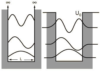e wavefunction ψ must go to zero at x=0 and x=L). Quantization of energy and position (namely, nodes at which the particle cannot exist) are directly to these quantum numbers, whose values are n=1, 2, ..., ∞, representing an infinite number of energy levels.

A particle in a finite box, however, can tunnel into the walls, in the same fashion that we saw earlier with the two barrier problems. Solving this system is not difficult but, unfortunately, has no analytical solution and must be solved either numerically or, as was done in class, graphically. On the other hand, the wavefunctions are essentially just those from the infinite box but are allowed to bleed into the wall (with the caveat that higher energy states tunnel further than the lower energy states). To summarize the major differences between the particle in a finite box and one in an infinite box:

• only a finite number of energy levels exist [called bound states]
  
• tunneling into the barrier is possible
  
• higher energy states are less tightly bound than lower states
• a particle given enough energy can break free [in other words, unbound]

The next quantum system to investigate is the one-dimensional harmonic oscillator, whose potential [from Hooke's Law] is V=1/2kx². Plugging this into the Schrödinger Equation leads to, after some well-chosen substitutions, a differential equation solved by Hermite in the mid-1800's, and we obtain the wavefunction: ψ(x) = N_vH_ve^-q2/2, where q = αx, v is the quantum number [v=0, 1, ...] and H_v are the Hermite polynomials. Here we see energy quantization as well, giving E = (v + 1/2)hbarω. This quantum system is the only one to exhibit constant spacing but other results mirror those seen in prior examples: tunneling into classically forbidden zones (where x represents displacement from equilibrium rather than position), a nonzero ground state energy as well as the existence of nodes.

One important distinction from the particle in a box result is that the peaks in the wavefunction are not uniform. For example, for v=2 and larger, it is clear that outside peaks (representing larger displacement from x=0) have higher probability than inside peaks. As n gets large, we see another clear example of the correspondence principle.

Obits

Wow, first John Wheeler on Sunday and today Edward Lorenz. A sad week for science...

Finite Barrier Tunneling and the Uncertainty Principle

When a quantum particle encounters a discontinuity in the form of a finite barrier, there is a nonzero probability that it will be transmitted to the other side of the barrier. In fact, as the graphic at right shows, the wavefunction bifurcates into a reflected as well as a transmitted part, a decidedly nonclassical and headscratching result (remember the Copenhagen interpretation) -- the three curves, by the way, show the real and imaginary parts of the wavefunction as well as the probability density.

Such tunneling phenomena are found throughout physics, chemistry and molecular biology, from explanations of alpha and beta decay to kinetic isotope effects and electron and proton transport in enzymes. It is likely that all redox chemistry has a tunneling component, which becomes even more prominent as the temperature falls.

Before moving onto the next quantum system, the particle in a finite box, we take a moment to consider one of the most important discoveries in all of quantum mechanics, the uncertainty principle. Heisenberg, in his development of matrix mechanics (an alternate description of quantum behavior, using matrices instead of differential operators), he discovered that some matrices did not commute, particularly those for momentum and position. After a little work he was able to demonstrate that this placed limits on the knowledge of the corresponding observable and we were doomed to indeterminacy. In particular, he found that ∆x∆p ≥ hbar/2, where ∆x and ∆p are the standard deviations of position and momentum.

Classically these values are zero: we can always know the position of, say, a marble and its velocity (and hence its momentum). At the quantum scale, these values are nonzero and, more baffling, are connected. The more precise we can nail down the position, for example, the less we will know about its momentum (and vice versa). Clearly we have to give up the Newtonian idea of knowing the trajectory of any quantum particle. This is not really an issue with measurement itself but rather a fundamental description of the quantum nature of the universe.

As we will see there are a number of uncertainty principles and they arise whenever we have noncommutative operators. In other words, whenever [a,b] ≠ 0, we will have an uncertainty principle in the corresponding observables: ∆a∆b ≥ hbar/2.

Solving the Schrödinger Equation

To understand simple quantum systems and solving the appropriate Schrödinger equation, we move through increasingly complicated systems. Whenever such an equation is solved, we typically acquire the wavefunction ψ and expressions for the energy E.

system I
A free particle in a potential of V=0. The general solution to the SE can be expressed two ways, both of which are commonly used: ψ = A'sin(kx) + B'cos(kx) or ψ = Ae^ikx+Be^-ikx (the latter used when we care about which direction the particle is moving, the former when we want mathematical nicety). The wavevector k is equal to √2mE/h_bar.

system II
A particle in a potential of V=V_o. The general solutions are the same as in system I, except here k=√2mT/h_bar, where T is the kinetic energy. Since k = 2π/λ, we can see that the wavelength decreases as T increases.

system III
A particle confined to an infinite one-dimensional square well (V=0 inside). Here the wavefunctions are ψ_n=√2/L sin(nπx/L) and the energies are E_n=n²h²/8mL² where n = 1, 2, ...

Three nonclassical results arise: (a) quantization of energy, which arises from putting constraints on the wavefunction (requiring it to go to zero at x=0 and x=L), (b) appearance of nodes, which limit positions at which a particle can exist in a box, and (c) nonzero ground-state (also known as the zero point energy). This "particle in a box" problem has been used to model, among other things, electrons in conjugated molecules and electrons in wires. Moreover it is one of the easier quantum systems to solve that simply demonstrates the important concepts of quantization of energy, nodes, normalization. and the correspondence principle.

system IV
A particle confined to a two-dimensional infinite box (V=0, ∞ outside). Using the method of separation of variables, we assume that ψ=X(x)Y(y), put it back into the SE and, while crossing our fingers, hope that it will crack into two equations. Fortunately it does just that, giving multiplicative wavefunctions ψ(x,y) = 2/√L_xL_y sin(n_xπx/L_x)sin(n_yπy/L_y) and additive energies E=h²/8m(n_x²/L_x² + n_y²/L_y²). The solution clearly gives two quantum numbers (arising from two dimensions/coordinates) and the possibility of degeneracy arises, where two or more distinct wavefunctions have the same energy. The extension to three-dimensional boxes (or higher) should be straightforward to write down without solving the Schrödinger Equation from scratch.

system V
The barrier problem, in which a particle experiences a discontinuity in potential; for example, going from V=0 to V=V_o at x=0. Fortunately we know these solutions from systems I and II and can write them down immediately: ψ_I = Ae^ikx+Be^-ikx and ψ_II = Ce^ikx+De^-ikx. We note, however, since there is nothing to reflect the particle back once it passes the barrier, that D=0.

To make these wavefunctions plausible we must "glue" them together; in other words, we must make them connect [ψ_I(x=0)=ψ_II(x=0)] and connect smoothly [dψ_I/dx(x=0)=dψ_II/dx(x=0)].

When we calculate the transmission probability T=C*C/A*A, we find that it can never equal unity (meaning that there will always be some amount of reflection from a barrier. Also, when the particle energy E is less than the potential V_o we find that the particle can exist in the barrier to a finite, though exponentially decaying degree. Such penetration into the classical forbidden area is called tunneling, a very important phenomenon in quantum chemistry and the subject of the next lecture.

Extracting Information from a Wavefunction

In a given quantum system, the wavefunction ψ is said to contain all of the information knowable about that system; the only trick is getting it out and that is where operators come in. A fundamental postulate of quantum mechanics is that every measurable quantity, whether it is total energy, angular momentum, position, etc, has a corresponding quantum mechanical operator. The position and momentum operators are of particular importance since nearly all other relevant operators can be constructed from them.

Sometimes when an operator operates on a wavefunction we get, as a result, a constant multiplied by that wavefunction; in other words, an eigenvalue equation. When we obtain such an eigenvalue equation, the corresponding eigenvalue represents the only value for that observable. When we do not obtain an eigenvalue equation, our observables will not be singly-valued; in other words, the observable will span a range of values.

Although we hope for eigenvalue equations, we can still calculate values for observables, but we are doomed to talk only about probabilities. For example, when the position operator x doesn't give an eigenvalue, we can refer instead to the expectation value for x (represented by and often referred to as the average value).

Wave Mechanics and the Schrödinger Equation

Two of the aforementioned failures of classical physics lead directly to the earthshaking matter-wave hypothesis of deBroglie: Einstein had demonstrated the wave-particle duality of light through his theory of the photon and Bohr, through his solar-system model of the hydrogen atom, hinted at the quantization of electron energies (we will cover his model more thoroughly when we get to atoms but the basics are well known to anyone who has taken general chemistry). Using a few equations from special relativity, deBroglie not only assumed that all matter had wavelike (as well as particle) properties, but in 1923 he derived a very simple relationship between wavelength and momentum: λ=h/p. In doing so, he essentially bridged what is now called the "old quantum theory", which lasted for about twenty years, to the much more successful (and abstract and perhaps unsettling) quantum mechanics of Schrödinger and Heisenberg.

The mathematical description of traveling and standing waves, utilizing terms like amplitude, frequency, wavelength, wavevector and period, had already been well-established by the mid-19th century. The Schrödinger Equation, though invoking these same mathematical constructs, can not be derived from any theory: it is simply asserted as a complete description of the physics of small particles. When the potential experienced by a particle of mass m is time-independent, we get the following equation (which should be committed to memory for any student studying quantum mechanics):
What changes from problem to problem is the nature of the potential V and the coordinate system, which will change the form of the laplacian operator and what is obtained when the Schrodinger Equation is solved are mathematical descriptions of the wavefunction ψ and the energy E. We will soon see that ψ contains all the possible information about the quantum system but what is not so trivial is getting that information out. For that we will need the ideas of operator alebra and eigenvalue equations.

Next up: Descriptions of the momentum and position operators, followed by the very important hamiltonian operator, and our first solution to the Schrödinger Equation, the so-called particle in a box problem.

The Failures of Classical Physics

Quantum mechanics represents such a break from classical [Newtonian] mechanics and is still -- 100 years later -- so anti-intuitive, that we pause to look at three experiments/observations that demonstrated the cracks arising back then in classical physics: blackbody radiation, the photoelectric effect and atomic spectra.

At room temperature a blackbody [that is, a body which reflects no incident light] emits infrared light but, as it is heated, this radiation moves into the visible spectrum, beginning at orange and increasing towards bluish white. Using classical theories, Rayleigh and Jeans derived an equation for the spectral density (energy density per unit frequency per volume) as a function of frequency. This model, however, was a horrible failure in that it did not correlate at all with experimental results, leading instead to a spectral density that reaches infinity in the ultraviolet regime [leading to what we now call the ultraviolet catastrophe].

Max Planck, in 1900, solved the problem (and unwittingly triggered the quantum revolution) by assuming that the blackbody was made of oscillators that could emit energy only in packets of nhν, where n is a nonnegative integer and h is a constant (now called Planck's constant). This assumption leads directly to the Planck distribution, which fit the experimental data perfectly when h=6.626E-34 Js. He spent the next few years unconvinced that h had much physical meaning and was not a strong supporter of the quantum theory, but by the time Einstein and Bohr hopped aboard, the train had left the station.

The photoelectric effect, in which light shined onto a metal induces a current [but only if its frequency is above some threshold], was also a mystery awaiting an explanation. Einstein's radical 1905 postulate, for which he won the Nobel Prize in Physics, was that light was comprised of corpuscular [particle-like] packets of energy hν called photons. The photoelectric effect could then be understood as a simple collision between two particles -- the photon and the electron in the metal. If the frequency of light were high enough, it would have an energy sufficient to overcome the binding energy [called the work function] of the electron to the metal. Einstein also, to his chagrin years later, the idea of the wave-particle duality, which is one of the more fundamental and vexing aspects of quantum mechanics.

When the emitted light of a heated gas is separated through a prism, a line spectrum occurs [as opposed to the continuous rainbow-type spectrum seen from sunlight]. The wavelengths of these lines could be fit to the Rydberg formula but, since it is simply an empirical formula and not based on any underlying theory, it further demonstrated the problems of classical physics. The Rydberg formula was eventually theoretically derived in the work of Bohr, whose model of the hydrogen atom we will visit a little later.

Much of what we have described thus far, including the early work of Planck, Einstein and Bohr, is generally referred to as the old quantum theory. One giant step further, spurred on by the work of deBroglie, is quantum mechanics, which we will visit next.

pchem III is days away

four experiences down but a final left

I have posted a final topic sheet and a final equation sheet. Not only does the latter have most of the important mathematical relations we studied in class but also makes a great wrapping paper. Solutions to hw.6 went up a couple of days ago...

A note on hw.6 problem 03 => answers for (a) and (b) were inadvertently switched: The faster rate has the larger k.

Thanks for all your hard work this quarter. Our final on Friday will likely be your last before spring break (sadly I have another one immediately afterwards) so make sure you get a good rest before returning for pchem III, perhaps the best of all the pchems.

To the three of you escaping to go on the boat, we'll miss you! [tear]

On the road to equilibrium

Equilibrium was an important theme last quarter, forming the basis of the ideas of reversibility and nearly all of the rest of thermodynamics. This quarter equilibrium has shown itself as the state towards which transport properties and chemical kinetics approach. As we solve the mechanism of opposing/reversible reactions, we are bridging the worlds of thermodynamics and kinetics.

For the reaction A ↔ B, we can readily write the differential equations for A and B:

dA/dt = - k_fA + k_rB
dB/dt = + k_fA - k_rB

Assuming that there is only A initially, we can state that A_o = A+B, or B = A_o - A, which, when plugged into equation 1 above, makes it integrable (two variables only). The solutions are:

A = A_o[ (k_r + k_fe^-(kf+kr)t)/(k_r + k_f) ]
B = A_o[ 1 - (k_r + k_fe^-(kf+kr)t)/(k_r + k_f) ]

To connect to equilibrium, we recognize that A(∞)=A_eq and that B(∞)=B_eq:

A_eq = A_o[ k_r/(k_r + k_f) ]
B = A_o[ k_f/(k_r + k_f) ]

Cool, from just kinetics we can predict equilibrium quantities of A and B. But not only that, we can take their ratio and obtain the equilibrium constant:

K = k_f/k_r

Remarkably, this is the result for all reversible reactions ( 2A ↔ B, 3A ↔ 2B, etc) and is called the principle of microscopic reversibility.

More complicated mechanisms can be understood as combinations of branching, sequential and opposing reactions. When intermediates are reactive, we can often use the steady-state approximation, which says that dI/dt ≅ 0. This allows us to more easily obtain rate laws from mechanisms without solving elaborate series of differential equations that take lots of time and make your soul cry.

Chemical Kinetics and You

The last time-dependent phenomenon we study this quarter is chemical kinetics or the change of chemical identity as a function of time. In many ways this is an extension of transport phenomena except that the physical space over which it flows has been replaced with a chemical space. It is also one of the subfields of physical chemistry that ties most strongly with organic chemistry and biochemistry.

We can track the extent of the general reaction aA( ) + bB( ) → cC( ) + dD( ) by tracking A, B, C or D with whichever experimental techniques are most convenient, as in optical activity, absorbance or nmr. Formally, the number of moles of species i at any time t will be tethered to the extent of reaction ξ by the following relation:

n_i = n_o,i + ν_iξ

It is through the extent of reaction that we define the [extensive] rate of reaction: Rate = dξ/dt. To obtain the intensive rate, we divide by the volume to get R = Rate/V. This is why, incidentally, that mol L^-1 is the natural unit of kinetics (instead of, say, activity which establishes the basis of most of solution thermodynamics).

Several properties affect the rate of a reaction, which include (a) concentration, (b) temperature, (c) physical state and (d) presence of catalysts. The concentration dependence is most important, most common and, unfortunately, most complicated -- we are decades away, if that, from being able to predict the behavior of even the simplest reactions from their stoichiometry.

Rates of reaction are dependent on the frequency of collisions, which is in turn dependent on the concentration of reactants, and we model this mathematically with a rate equation (aka rate law): R = kA^αB^β where α and β, the reaction orders with respect to A and B, are basically sensitivity factors to changes in concentration. The higher the order, the more sensitive that reaction is to changes in that reactant. The overall order is just the sum of the exponents, which are usually integers [like 1 or 2] or some simple fraction [like 3/2 or 1/4]. Incidentally, it will be through k itself that dependence on temperature and catalysis will appear, in the familiar, but empirical, Arrhenius equation.

Finding the rate law for a given reaction is the holy grail... once we have obtained it, we can in principle know the concentration of all reactants and products at any time afterwards (do you see the similarity to certain transport properties like, say, diffusion?). We discussed four methods of obtaining rate orders (and, hence, the general form of the rate law):

1. isolation method
2. method of initial rates
3. ntegrated rate laws, and
4. method of half-lives

When obtaining the integrated rate laws for 1st, 2nd and, finally, nth order, we discovered that the half-life is concentration dependent for all orders except for n=1. It is this concentration dependence that allows us to manipulate half-life experiments to give us information about the order of reaction, one of the most accurate methods currently at our disposal.

Another important goal in kinetics is the elucidation of the underlying mechanism for a given reaction, in which we conjecture a series of individual collisonal events [with molecularity 3 or less] that adds up to the overall stoichiometric reaction. It is only within these elementary step processes that we can correlate molecularity to reaction order (since, again, these represent actual collisions, not just stoichiometric bookkeeping).

Nearly all complex mechanisms are constructed from the following three elementary fragments:

branching/parallel: C ← A → B
sequential/consecutive: A → B → C
reversible/opposing: A ↔ B

In a multistep mechanism, all species are changing with time and it is the goal of pchem to know their functional forms, if possible [we will see shortly that this is easier said than done, since many mechanisms become mathematically intractable with just a few fragments].

For any mechanism, however, we can readilty write down the differential equations that could, in principle, be solved [analytically, numerically or graphically]. For instance, for the branching process above, we have three entities changing with time so we have three equations:

1. dA/dt = -k₁A - k₂A
2. dB/dt = k₁A
3. dC/dt = k₂A

For the consecutive reaction mechanism, we get a different set of three:

1. dA/dt = -k₁A
2. dB/dt = k₁A - k₂B
3. dC/dt = k₂B

In our next lecture, we will look at exact solutions to these two sets of coupled differential equations as well as reversible reactions [which will take us back to, of all places, equilibrium].

We have [finally] finished transport properties

In Chapter 17 we tackled many various transport properties, essentially extending the topics from pchem I [equilibrium thermodynamics] into time-dependent irreversible thermodynamics. Critical to this endeavor are the concepts of flux, gradient and curvature, each of which adds a unique parameter in which to describe nonequilibrium phenomena.

We first tackled ionic conduction, a logical extension of the electrochemical systems we examined in previous chapters [indeed, membrane potentials pointed the way towards this topic]. We saw how charged particles migrate under the influence of an electric field [an electrical potential gradient] and how Arrhenius and Kohlrausch stumbled onto the discovery that solutions were comprised of electrolytes, leading to mathematical expressions for both strong and weak electrolytes. (Arrhenius, incidentally, subscribed -- at least partially -- to a number of unusual theories). Ostwald contributed the dilution law, a clever method of obtaining dissociation constants by measuring the conductance of a series of dilutions of an electrolyte.

We can further characterize how fast an ion moves through a solvent under the influence of an external electric field from the equation s_i=u_iE, where u_i, the ionic mobility, is a parameter based on the identity of a particular ion (which also tells us something about how that ion interacts with water). Of special note is the Grotthuss mechanism, which helps explain why the mobilities of H⁺ and OH^-. Another helpful parameter is the transport number, or the fraction of the total current carried by a particular ion.

Shifting gears, we next tackled viscosity, the phenomena in which linear momentum is transported between sheets of flowing liquid, first described by Sir Isaac Newton in the 18th century. In fact, Newton's Law of Flow leads directly to the observation that, for laminar flow, the velocity profile through a tube is parabolic (with the greatest velocity at R=0). We can use this result in turn to verify Poiseulle's Law, which associates flow rate dV/dt with the fluid viscosity. Newton's Law will not hold for nonlaminar [aka turbulent] flow, characterized by a high Reynolds number, or for thixotropic and/or dilatant fluids.

Our next transport property was one of enormous chemical and physiological importance, the diffusive motion of matter through a medium due only to thermal fluctuations. Brownian motion was observed shortly after the advent of the microscope and was further characterized by the random-walk theories of Smoluchowski and Einstein. A more sophisticated treatment can be found in Fick's 1st and, especially, 2nd Law of Diffusion. In class we looked at three solutions to the diffusion equation: case 1 [a solution of known concentration diffusing into pure solvent, in which we first encountered the erf function]; case 2 [a layer of particles initially sandwiched on either side by pure solvent]; case 3 [a point source of particles diffusing in 3d through pure solvent].

Before moving on, we pause to note that diffusion and viscosity are related through the shape-dependent frictional coefficient, as described in the Einstein relation: D=kT/ƒ. Earlier, George Stokes, a pioneer of fluid dynamics, had established ƒ for many shapes through theoretical and experimental studies of bodies falling through viscous fluids. Of particular importance is the equation for a sphere, ƒ = 6πηa.

Related to diffusion is the motion of matter due to an external force, such as sedimentation [gravity and centrifugation] and electrokinesis [electric field]. Pioneered by Svedberg, analytical ultracentrifugation can reach simulated gravitational fields of nearly 1,000,000-g and is of considerable importance in polymer and biophysical characterizations of macromolecules. Sedimentation, when combined with diffusion information [often simultaneously in the AU], provides a method to experimentally measure the molar mass of a macromolecule/organelle/icky thing, a nontrivial parameter when dealing with conglomerates of particles with no discernible chemical formula. In addition, calculating its ƒ/ƒ_o (the ratio of the actual frictional coefficient to that if the molecule were spherical) gives us a unique shape parameter to describe its sphericality [or not].

Lastly we examined electrokinetic effects, a brief foray back into the world of electrochemistry. In these phenomena [notably electroosmosis and electrophoresis], the particle size is much larger, giving rise to an interface between the particle and the solution. Two models of this interface were discussed: the Helmholtz model [fixed double layer] and the Gouy-Chapman [diffuse double layer] model (truth in advertising: a third picture, the Stern model, which combines aspects of the Helmholtz and Gouy-Chapman models, is now preferred). Key to the diffuse double layer is the generation of a zeta potential, which is critical to explaining colloid stability and electroosmosis/electrophoresis.

Though not discussed in class, electroosmosis is likely to be of tremendous importance as microfluidic technologies gain maturity. Of course electrophoresis has become entrenched in biochemistry, biophysics and molecular biology, first with the development of the Tiselius tube and then with gel electrophoresis. Separation of macromolecules is possible by electrophoretic means if they possess different isoelectric points [that pH at which the electrophoretic mobility is zero, primarily arising from the balancing of cationic and anionic groups on the molecule].

My hope is that its obvious by now why a good grounding in pchem is so necessary to fully appreciate much of what we take for granted in chemistry and biochemistry [for instance, something as mundane as centrifugation] and even in many of our sister disciplines [like physiology and soil science].

And now, onwards to chemical kinetics, the last topic of this quarter, in which we study how chemical identity changes with time. And though you have studied this before in both general and organic chemistry, this time we will do it correctly... :) [with chewy calculus goodness].

Homework 3a Solutions

now that chemweb is back up, hw.3a solutions have been posted in the usual place

Electrochemical Potentials, Membrane Potentials

From last quarter in thermodynamics and the first half of this quarter, we have underscored the great importance of the chemical potential, noting that matter flows spontaneously from high to low μ. When these particles are charged, however, electrical work is performed in addition to chemical work. To take this into account, we transmogrify the chemical potential into the new-and-improved function, the electrochemical potential μ~ = μ + zFφ or

μ_i~ = μ_i° + RTlna_i + z_iFφ

From this thermodynamic function, we can derive most of the basics of electrochemistry:

• voltaic/galvanic cells use spontaneous redox reactions to generate voltage
• the cathode is the site of reduction and the anode is the site of oxidation
• electrons flow towards cathode making it the positive terminal
• standard reduction potentials use the conventional standard [E°(H⁺=0]
• cell potentials can be calculated by E°=E°_cathode-E°_anode
• cell notation is in form anode half cell || cathode half cell
• nonstandard potentials are calculated using Nernst eqn: E=E°-(RT/νF)lnQ
• pH is defined as -log(a_H+)
• concentration cells generate voltage using same half-cell at different concentrations
  

When a membrane separates two ionic environments, we again see that balancing the electrochemical potential leads to an electrical potential difference [the membrane potential]. Note again that, unfortunately, we are employing the term potential twice, the first being a form of Gibbs energy and the latter being a type of voltage. The membrane potential can be found from:

∆φ = (RT/z_iF)ln(a^α_i/a^β_i)

A more realistic scenario, called the Donnan effect, is scene we consider a membrane in which everything is permeable [ions, solvent] except for a macro-ion M. In addition to the electrochemical potential, the macro-ion will generate an osmotic pressure force on the α side, although this term is typically small enough to be neglected if the macro-ion is sufficiently dilute. With a half-page of work, we find the following relationships:

∆φ = (RT/z₊F)ln(Y)

where Y = m^α₊/m^β₊ (the concentration imbalance)

and, when M is dilute, Y ≅ 1 - z_Mm_M/2m^β

Salting-in and Salting-out

Since activity is a measure of the effective concentration of solute in a solution, it can be used to describe solubilities of slightly soluble solutes in ionic solutions. In other words, we can investigate the effects of ionic strength on solubility.

For example, since copper (II) sulfide is only somewhat soluble in water, we can write its dissolution as an equilibrium:

CuS(s) ↔ Cu²⁺(aq) + S^2-(aq)

The thermodynamically correct equilibrium constant is then

K_sp=a_Cua_S=γ_Cuγ_Sm_Cum_S=γ_±²K_sp^obs

The parameter K^obs is the observed (or apparent) equilibrium constant and will be the one that is measured by standard measurements like titration. Since this is a 1:1 ionic compound, K_sp is related to S, the molal solubility, by:

K_sp = S² and K_sp^obs = (S^obs)²

Combining the two equations above, we can solve for the ratio of solubilities:

S/S^obs = γ_±

Therefore, for mean activity coefficients less than one, we see an increase in solubility with respect to water [salting-in] and a corresponding solubility decrease when γ_± is greater than one [salting-out].

Debye-Hückel Theory

One of the problems that arises when treating the theory of ionic solutions is how exactly to deal with the activities of cations versus anions when both are always found together (all solutions are neutral). Recognizing this fact, we can define a mean activity coefficient in terms of the individual ion activity coefficients:

γ_± = [γ₊^ν+γ₊^ν-]^1/ν

But how do we obtain activity coefficients without going through tedious cryoscopic or electrochemical measurements? This is one of the results that the Debye-Hückel theory seeks to uncover. Before going through the details, we need a convenient way to describe how much a given solution can conduct electricity: the ionic strength I.

I = 1/2 Σ z_i² (m_i/m°) = 1/2 Σ z_i² m_i

Ionic strength is unitless so the last term above is basically a unitless molality.

Debye and Hückel proposed a simple model that they hoped would capture most of the behavior of ionic solutions. The assumptions:

1. an ionic atmosphere is established with many ions with valence z and radius a
2. the solvent is structureless with electric permittivity ε
3. the solution is dilute.

Several results were obtained via mind-bleeding statistical mechanics but among them were the Debye length τ_D, which is a measure of the effective range that ionic charges interact in this solution.

Another important result is the extended Debye-Hückel law:

lnγ_± = - |z₊z_-|αI^1/2/(1 + βaI^1/2)

which can also be written in ion activity form:

lnγ_i = -z_i²|αI^1/2/(1 + βaI^1/2)

As mentioned in class, this formula works quite well for dilute to moderately concentrated solutions (and is fairly bad past 0.25 m). For dilute solutions we can consider the limiting Debye-Hückel law:

lnγ_± = - |z₊z_-|αI^1/2

Since α=1.171 for water at 25°C, we can transmogrify any of these formulas to log₁₀ world. For example, the above equation becomes

logγ_± = -0.509 |z₊z_-|I^1/2 (aqueous solutions, 25°C)

Bjerrum, Mayer and Davies extended the Debye-Hückel formula so that it works for a wide range of ionic strengths (and remains the primary equation used in pchem today):

logγ_± = -0.509 |z₊z_-|(I^1/2/1+I^1/2 - 0.30I) (aqueous solutions, 25°C)

At different temperatures, new values for the Debye-Hückel parameter (the 0.509 value) would need to be calculated through α.

Tomorrow, salting-in and salting-out.

hw.1 corrections

For question 1, I mistakenly chose the chemical potential that was the lowest, not the highest.

Also, for question 12, the hydrogens on each benzoic acid are missing.

Activity Gets Promoted

Before grappling with the chemical potentials of ionic solutions, we took a moment to update the colligative property formulas for ionic solutes. Since these properties depend not on what is dissolved in solution but how much, the fact that salts break into ions needs to be addressed, which is accomplished by i, the van't Hoff factor:

• freezing point depression: ∆T_f=iK_fm₂
• boiling point elevation: ∆T_b=iK_bm₂
• osmotic pressure: Π=iM₂RT

where i = (actual number of free particles)/(number before dissociation).

For very dilute solutions, i is approximately equal to the number of ions in the formula (i=2 for KCl, i=3 for Na₂SO₄, etc.). As the concentration increases, the actual van't Hoff factor will be less (sometimes very much so) than these stoichiometrically derived values. We also saw that we could relate i to the degree of dissociation α by the formula α=(i-1)/(ν-1).

Although earlier we defined the chemical potential of a solution in terms of the Raoult's standard state [purity and mole fraction], it is more convenient to use a standard state based on molality:

For a solute in an ideal solution: μ_i = μ°_i + RT lnm_i
For a solute in a real solution: μ_i = μ°_i + RT lna_i

Henceforth the symbol ° will mean 1 bar for gases and 1 m for solutions. Since we now have six different chemical potential expressions [ideal gas, real gas, ideal solution, real solution, liquid, solid] it is customary to promote the idea of activity so that it covers all possibilities. We will then use a general expression μ_i = μ°_i + RT lna_i with the following mappings:

• ideal gas: a_i = P_i [partial pressure]
  
• real gas: a_i = f_i [fugacity]
  
• ideal soln: a_i = m_i [molality]
  
• real soln: a_i = a_i [activity]
  
• liquid: a_i = 1 [assuming normal pressure]
  
• solid: a_i = 1 [assuming normal pressure]

Now, for any reversible chemical reaction aA( )+bB( ) ↔ cC( )+dD( ) we can construct reaction quotient and equilibrium constant expressions immediately in terms of the relevant activities.

Tomorrow we will go through the powerful Debye-Hückel theory, which gives considerable insight into ionic solutions, including a method to calculate activity coefficients. Also, next hw set..

The Born Model of Solvation

Since ionic compounds, when dissolving, produce a cationic and anionic pair, the thermodynamics of ionic solutions becomes complicated in that values for a single ion are unknowable. Conventional values are obtained by assigning ∆_fG°[H⁺]=0 for all temperatures and then calculating every other ion value with respect to that reference. This process works well in Hess' Law-type calculations as long as we don't assign meaning to individual ion values (particularly true for negative S_f° values).

Though ultimately less successful, we can gain a lot of insight into the solvation process by attempting to derive the thermodynamic values from scratch, that is, from first principles. In the Born model, we imagine a hard-sphere of radius r being charged up from 0 to a final value q. The difference between the work of charging this ion in the medium of choice and a vacuum will be taken as ∆_solvG_i° for ion i.

Recalling that the infinitesimal work of charging is dw=φdq and the electric potential is φ=q/4πεr, we obtain for 1 mole of ions, after integrating and substituting q=ze:

∆_solvG_i°=z²e²N_A/8πε_or(1/ε_r-1)

Since the dielectric constant is greater than 1 for all materials, the solvation of any ion is a spontaneous process in any solvent.

Focusing on 298K water as the solvent leads us to gibbs energy of hydration:

∆_hydG°=-68.6z²/r

A test of the Born model can be obtained by plotting experimental ∆_hydG° values versus z²/r for a bunch of ions and see whether or they not they track along a line of slope –68.6. As seen in class, most univalent ions generally agree with the Born results but polyvalent ions deviate appreciably, especially as the valence z gets large.

This is a good example of how physical chemistry works: Propose a model that is as simple as possible and see how much of the chemical behavior is captured. When it fails for some cases, go back and examine the assumptions (and tweak and repeat). In this model, the assumption of the aqueous solvent being structureless (that is, a continuum) is likely the culprit. Indeed, we saw that many of the high-valence ions seem to be tracking along a line in which the dielectric constant was approximately 2 (indicative of a case in which the mobility of water has been decreased to the point that it acts effectively as a nonpolar substance). An additional deviation from the Born model, not discussed much in class, arises from ions that are highly polarizable and would therefore not be adequately treated as a hard-sphere.

Many models exists treating the solvent as a molecular entity exist and experiments and simulations support the theory that an ion in solution produces a hydration sphere encompassing 4-8 water molecules (the actual number being a function of ionic size). Indeed, femtosecond laser studies provide hydration lifetimes for water molecules in the presence of a particular ion. Some ions with high charge densities have very long lifetimes, supporting the idea that water in those cases has been effectively locked immobilized.

Though the underlying explanation has not been fully developed, we can experimentally verify that some ions in solution increase the viscosity when compared to water. These kosmotropic ["structure-making"] ions include Li⁺, Na⁺ and F^-. Analogously, viscosity is decreased by chaotropic ["structure-breaking"] ions like Rb⁺, Cs⁺ and NO₃^-.

On Wednesday, a brief return to colligative properties (to adjust them for ionic solutions) before tackling chemical potentials of ionic solutions, activity and the Debye-Huckel theory.

Chemical Potential Leads to More Goodies

Colligative properties, those that depend not on the identity of a solute but only on how much is dissolved, had been known experimentally for years before an underlying theory was established. We typically discuss four such properties of solutions (and are compared to the corresponding pure solvent): vapor pressure lowering, freezing point depression, boiling point elevation and osmotic pressure.

It should be apparent from Monday's lecture that vapor pressure lowering for ideal solutions is an obvious consequence of Raoult's Law, although all solutions experience the phenomenon (which is due to the fact that the chemical potential is lower for a solution than it is for the solvent: μ₁(soln)=μ*₁(l)+RTlnX₁). But all four of these phenomena are explained by setting the appropriate chemical potentials equal (where we designate 1 as the solvent and 2 as the solute):

vp lowering: μ₁(soln) = μ₁(g)
fp depression: μ₁(soln) = μ₁(s)
bp elevation: μ₁(soln) = μ₁(g)
osmotic pressure: μ₁(l) = μ₁(soln) + ΠV_m

Using some math elegance with a few key assumptions (like ∆_transH being relatively constant and the solution dilute), we are able to obtain the experimentally obtained formulae familiar to students of general chemistry:

bp elevation: ∆T_b=K_bm where [ebullioscopic constant] K_b=RM₁T_b²/∆_vapH
fp elevation: ∆T_f=K_fm where [cryoscopic constant] K_f=RM₁T_f²/∆_fusH
osmotic pressure: Π=MRT

Since we have thus far dealt only with molecular [nonionic] solutions, we needed to refresh some concepts from basic electrostatics [coulomb's law, electric permittivity, dielectric constants] before moving onto ionic solutions, which can be radically different (and never truly ideal).

Ideal Solutions, Raoult's Law and Azeotropes

We begin pchem II by examining the behavior of solutions. In Chapter 9 we briefly study nonelelectrolyte solutions and then, in Chapter 10, focus on the more common ionic solutions and activity.

Ideal solutions are those solutions in which components A and B attract each other to the same degree that they attract themselves and would thus posses zero values for ∆_mixV and ∆_mixH. Examples of solutions that approximate ideality are hexane:heptane and CCl₄:SiCl₄ (approximately the same structure and intermolecular forces).

Though originally obtained experimentally, Raoult's Law can be derived from chemical potentials and describes how the vapor pressure of a solution compares to that of the pure solvent: P_i=X_iP*_i. Since this relationship only works for ideal solutions, some have argued that it could just as easily be used as a second definition of what constitutes ideality in a solution.

In a binary ideal solution, if both components are volatile they will both contribute to the overall vapor pressure: P=X₁P*₁+X₂P*₂. Using the fact that mole fractions add up to 1, it is easy to obtain the equation P=P*₂+(P*₁-P*₂)X₁. Clearly, if we were to plot the vapor pressure versus composition, we obtain a line connecting the pure vapor pressures (which represents the liquid-vapor coexistence curve for this P-X phase diagram).

With a little bit of work, we also obtain an expression for the total vapor pressure in terms of Y_i, the vapor-phase mole fraction, whose plot is squashed-hyperbolic and also shown above. Both are typically superimposed together to form a P-Z (pressure-composition) diagram.

A generally more useful diagram however is one that plots the boiling temperature rather than the vapor pressure on the vertical axis. Such plots are useful to explain the physical chemistry of simple and fractional distillation. For example, this T-Z diagram shows the analysis of an ideal benzene:toluene solution in which X_benzene=0.20 initially. As the solution is slowly heated, the temperature eventually reaches the coexistence curve at about 375°C. The corresponding vapor-phase mole fraction is found by drawing a straight line across to the other coexistence curve (which represents Y values): Here we find a value of 0.36 which is clearly richer in benzene than the original solution. If we were to simply remove this vapor and condense it, we'd get a solution in which X_benzene=0.36 and we could start the process again. By using a Vigreaux condensor, however, we can do it all in one process.

When solutions possess considerable nonideality, kinks in the T-Z diagram can occur, leading to azeotropes (solutions that boil at constant temperature). Positive deviations from Raoult's Law lead to minimum boiling point azeotropes while negative deviations lead to maximum boiling point azeotropes. Azeotropic pairs, like the famous ethanol:water solution, can not be completely separated by distillation methods.